Plotting tools for BiCop objects

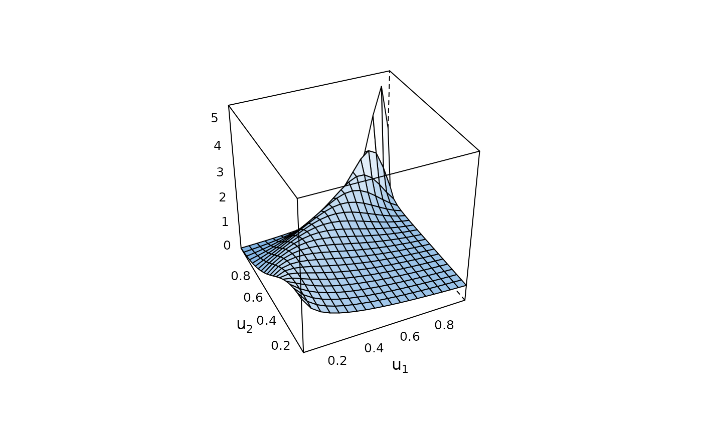
There are several options for plotting BiCop objects. The density of a bivariate copula density can be visualized as surface/perspective or contour plot. Optionally, the density can be coupled with standard normal margins (default for contour plots). Furthermore, a lambda-plot is available (cf., BiCopLambda()).

# S3 method for BiCop
plot(x, type = "surface", margins, size, ...)

# S3 method for BiCop
contour(x, margins = "norm", size = 100L, ...)

Arguments

x: BiCop object.
type: plot type; either "surface", "contour", or "lambda" (partial matching is activated); the latter is only implemented for a few families (c.f., BiCopLambda()).
margins: only relevant for types "contour" and "surface"; options are: "unif" for the original copula density, "norm" for the transformed density with standard normal margins, "exp" with standard exponential margins, and "flexp" with flipped exponential margins. Default is "norm" for type = "contour", and "unif" for type = "surface".
size: integer; only relevant for types "contour" and "surface"; the plot is based on values on a \(size x size\) grid; default is 100 for type = "contour", and 25 for type = "surface".
...: optional arguments passed to contour() or wireframe().

Author

Thomas Nagler

Examples


## construct BiCop object for a Tawn copula
obj <- BiCop(family = 104, par = 2.5, par2 = 0.4)

## plots
plot(obj)  # surface plot of copula density

contour(obj)  # contour plot with standard normal margins

contour(obj, margins = "unif")  # contour plot of copula density

Arguments

See also

Author

Examples