Working with kdecopula objects
The function kdecop() stores it's result in object of class kdecopula.
The density estimate can be evaluated on arbitrary points with dkdecop();
the cdf with pkdecop(). Furthermore, synthetic data can be simulated with
rkdecop().
dkdecop(u, obj, stable = FALSE)

pkdecop(u, obj)

rkdecop(n, obj, quasi = FALSE)
Arguments
| u |
|
|---|---|
| obj |
|
| stable | logical; option for stabilizing the estimator: the estimated density is cut off at \(50\). |
| n | integer; number of observations. |
| quasi | logical; the default ( |
Value
A numeric vector of the density/cdf or a n x 2 matrix of
simulated data.
References
#' Nagler, T. (2018) kdecopula: An R Package for the Kernel Estimation of Bivariate Copula Densities. Journal of Statistical Software 84(7), 1-22 #' Geenens, G., Charpentier, A., and Paindaveine, D. (2017). Probit transformation for nonparametric kernel estimation of the copula density. Bernoulli, 23(3), 1848-1873. Nagler, T. (2014). Kernel Methods for Vine Copula Estimation. Master's Thesis, Technische Universitaet Muenchen, https://mediatum.ub.tum.de/node?id=1231221 Cambou, T., Hofert, M., Lemieux, C. (2015). A primer on quasi-random numbers for copula models, arXiv:1508.03483
See also
kdecop,
plot.kdecopula,
ghalton
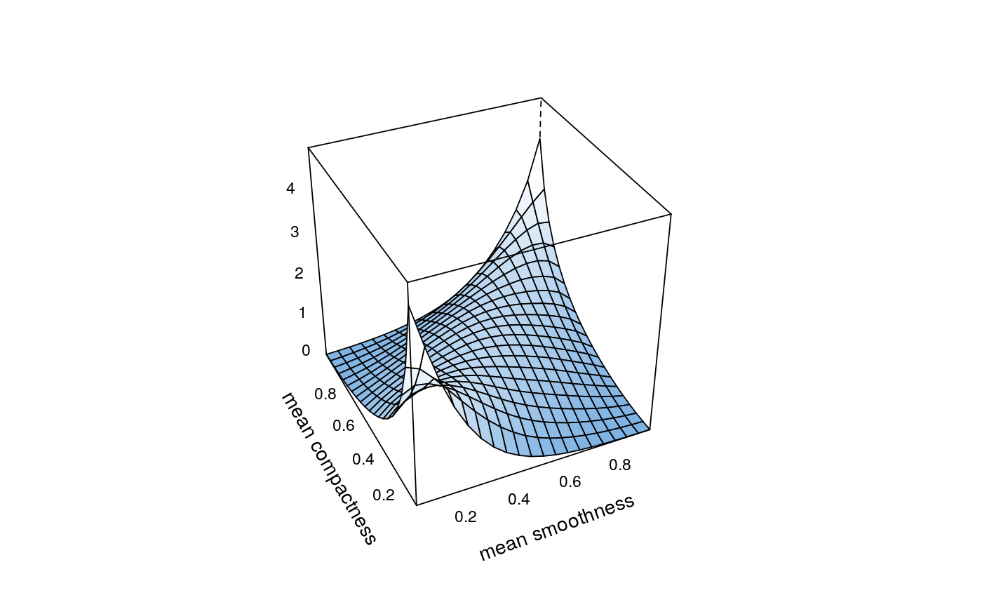
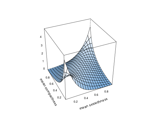
Examples
## load data and transform with empirical cdf data(wdbc) udat <- apply(wdbc[, -1], 2, function(x) rank(x) / (length(x) + 1)) ## estimation of copula density of variables 5 and 6 fit <- kdecop(udat[, 5:6]) plot(fit)## evaluate density estimate at (u1,u2)=(0.123,0.321) dkdecop(c(0.123, 0.321), fit)#> [1] 1.28916## evaluate cdf estimate at (u1,u2)=(0.123,0.321) pkdecop(c(0.123, 0.321), fit)#> [1] 0.09779868## simulate 500 samples from density estimate plot(rkdecop(500, fit))