Bivariate kernel copula density estimation

Based on samples from a bivariate copula, the copula density is estimated. The user can choose between different methods. If no bandwidth is provided by the user, it will be set by a method-specific automatic selection procedure. The related (d/p/r)kdecop functions evaluate the density and cdf or simulate synthetic data, respectively.

kdecop(udata, bw = NA, mult = 1, method = "TLL2nn", knots = 30,
  renorm.iter = 3L, info = TRUE)

Arguments

udata	`nx2` matrix of copula data.
bw	bandwidth specification; if `NA`, `bw` is selected automatically (see Details); Otherwise, please provide `"T", "TLL1", "TLL2"`: a $2x2$ bandwidth matrix, `"TLL1nn", "TLL2nn"`: a list with (named) entries `B`, `alpha`, and `kappa`, `"TTCV", "TTPI"`: a numeric vector of length four containing $(h, \rho, \theta_1, \theta_2)$, c.f. Wen and Wu (2015), `"MR", "beta"`: a positive real number.
mult	bandwidth multiplier, has to be positive; useful for making estimates more/less smooth manually.
method	`"T"`: transformation estimator based on classical bivariate kernel estimation (e.g., Geenenens et al., 2014), `"TLL1"`: transformation estimator with log-linear local likelihood estimation (Geenenens et al., 2014), `"TLL2"`: transformation estimator with log-quadratic local likelihood estimation (Geenenens et al., 2014), `"TLL1nn"`: transformation estimator with log-linear local likelihood estimation and nearest-neighbor bandwidths (Geenenens et al., 2014), `"TLL2nn"`: transformation estimator with log-quadratic local likelihood estimation and nearest-neighbor bandwidths (Geenenens et al., 2014), `"TTPI"`: tapered transformation estimator with plug-in bandwidths (Wu and Wen, 2015), `"TTCV"`: tapered transformation estimator with profile cross-validation bandwidths (Wu and Wen, 2015), `"MR"`: mirror-reflection estimator (Gijbels and Mielniczuk, 1990), `"beta"`: beta kernel estimator (Charpentier et al., 2006), `"bern"`: Bernstein copula estimator (Sanchetta and Satchell, 2004); the coefficients are adjusted by the method of Weiss and Scheffer (2012).
knots	integer; number of knots in each dimension for the spline approximation.
renorm.iter	integer; number of iterations for the renormalization procedure (see Details).
info	logical; if `TRUE`, additional information about the estimate will be gathered (see Value).

Value

The function kdecop returns an object of class kdecopula that contains all information necessary for evaluation of the estimator. If no bandwidth was provided in the function call, the automatically selected value can be found in the variable object$bw. If info=TRUE, also the following will be available under object$info:

likvalues

Estimator evaluated in sample points

loglik

Log likelihood

effp

Effective number of parameters

AIC

Akaike information criterion

cAIC

Bias-corrected version of Akaike information criterion

BIC

Bayesian information criterion.

The density estimate can be evaluated on arbitrary points with dkdecop; the cdf with pkdecop. Furthermore, synthetic data can be simulated with rkdecop, and several plotting options are available with plot and contour.

Details

We use a Gaussian product kernel function for all methods except the beta kernel and Bernstein estimators. For details on bandwidth selection for a specific method, see: bw_t, bw_tll, bw_tll_nn, bw_tt_pi, bw_tt_cv, bw_mr, bw_beta, bw_bern.

Kernel estimates are usually no proper copula densities. In particular, the estimated marginal densities are not uniform. We mitigate this issue by a renormalization procedure. The number of iterations of the renormalization algorithm can be specified with the renorm.iter argument. Typically, a very small number of iterations is sufficient.

Note

The implementation of the tapered transformation estimator ("TTPI"/"TTCV") was kindly provided by Kuangyu Wen.

References

Geenens, G., Charpentier, A., and Paindaveine, D. (2017). Probit transformation for nonparametric kernel estimation of the copula density. Bernoulli, 23(3), 1848-1873. Wen, K. and Wu, X. (2015). Transformation-Kernel Estimation of the Copula Density, Working paper, http://agecon2.tamu.edu/people/faculty/wu-ximing/agecon2/public/copula.pdf Gijbels, I. and Mielniczuk, J. (1990). Estimating the density of a copula function. Communications in Statistics - Theory and Methods, 19(2):445-464. Charpentier, A., Fermanian, J.-D., and Scaillet, O. (2006). The estimation of copulas: Theory and practice. In Rank, J., editor, Copulas: From theory to application in finance. Risk Books. Weiss, G. and Scheffer, M. (2012). Smooth Nonparametric Bernstein Vine Copulas. arXiv:1210.2043 Nagler, T. (2014). Kernel Methods for Vine Copula Estimation. Master's Thesis, Technische Universitaet Muenchen, https://mediatum.ub.tum.de/node?id=1231221

Examples


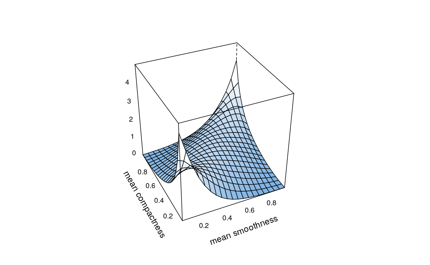
## load data and transform with empirical cdf
data(wdbc)
udat <- apply(wdbc[, -1], 2, function(x) rank(x) / (length(x) + 1))

## estimation of copula density of variables 5 and 6
fit <- kdecop(udat[, 5:6])
summary(fit)
#> Kernel copula density estimate (tau = 0.49)
#> ------------------------------
#> Variables:    mean smoothness -- mean compactness 
#> Observations: 569 
#> Method:       Transformation local likelihood, log-quadratic (nearest-neighbor, 'TLL2nn') 
#> Bandwidth:    alpha = 0.5689854
#>               B = matrix(c(0.71, 0.71, -0.71, 0.71), 2, 2)
#> ---
#> logLik: 190.97    AIC: -357    cAIC: -356.4    BIC: -302.85 
#> Effective number of parameters: 12.47
plot(fit)
contour(fit)

## evaluate density estimate at (u1,u2)=(0.123,0.321)
dkdecop(c(0.123, 0.321), fit)
#> [1] 1.28916

## evaluate cdf estimate at (u1,u2)=(0.123,0.321)
pkdecop(c(0.123, 0.321), fit)
#> [1] 0.09779868

## simulate 500 samples from density estimate
plot(rkdecop(500, fit))  # pseudo-random
plot(rkdecop(500, fit, quasi = TRUE))  # quasi-random