An R package that provides functionality to fit and simulate from stationary vine copula models for time series.
The package is built on top of rvinecopulib and univariateML.
Installation
Install the released version from CRAN.
install.packages("svines")Install the development version from GitHub with remotes.
# install.packages("remotes")
remotes::install_github("tnagler/svines")
Usage
For detailed documentation and examples, see the package website.
Use svine() for observed data: it estimates the marginal distributions and the S-vine copula. Use svinecop() when the margins have already been transformed to approximately uniform pseudo-observations.
Fitting models
fit <- svine(returns, p = 1)  # Markov order 1
summary(fit)
#> $margins
#> # A data.frame: 2 x 5
#>  margin    name          model                         parameters loglik
#>       1 Allianz Skew Student-t 0.00039, 0.01589, 5.45534, 0.91785   1382
#>       2     AXA Skew Student-t 0.00052, 0.02089, 4.35198, 0.90611   1260
#>
#> $copula
#> # A data.frame: 5 x 10
#>  tree edge conditioned conditioning var_types family rotation   parameters df
#>     1    1        3, 2                    c,c      t        0 0.037, 4.893  2
#>     1    2        2, 1                    c,c      t        0   0.86, 3.48  2
#>     2    1        4, 2            3       c,c    joe       90          1.1  1
#>     2    2        3, 1            2       c,c  indep        0               0
#>     3    1        4, 1         2, 3       c,c      t        0 0.079, 8.994  2
#>     tau
#>   0.023
#>   0.662
#>  -0.033
#>   0.000
#>   0.051
contour(fit$copula)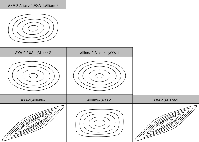
Simulation
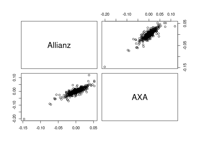
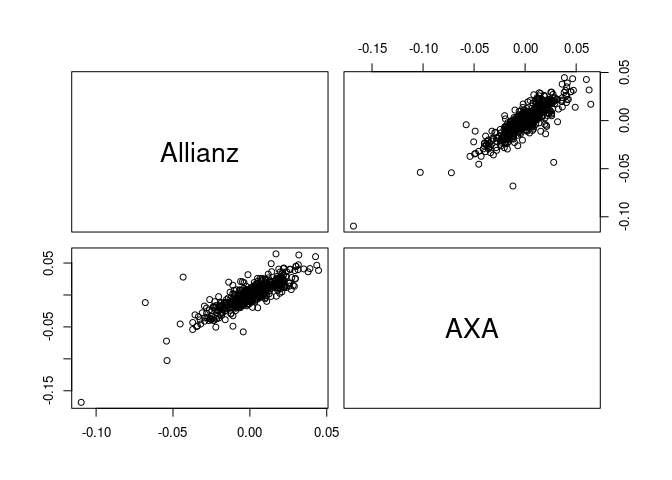
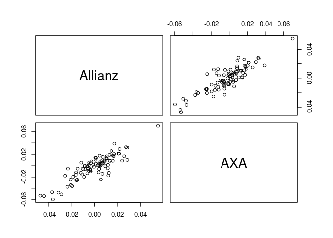
svine_sim() can be used in two different ways:
Standard errors
To generate bootstrap replicates with the one-step block multiplier bootstrap, use
set.seed(2026)
models <- svine_bootstrap_models(2, fit)
summary(models[[1]])
#> $margins
#> # A data.frame: 2 x 5
#>  margin    name          model                         parameters loglik
#>       1 Allianz Skew Student-t 0.00057, 0.01437, 7.22824, 0.97850     NA
#>       2     AXA Skew Student-t 0.00065, 0.01842, 5.29395, 0.98127     NA
#>
#> $copula
#> # A data.frame: 5 x 10
#>  tree edge conditioned conditioning var_types family rotation    parameters df
#>     1    1        3, 2                    c,c      t        0 -0.022, 5.380  2
#>     1    2        2, 1                    c,c      t        0    0.84, 2.99  2
#>     2    1        4, 2            3       c,c    joe       90             1  1
#>     2    2        3, 1            2       c,c  indep        0                0
#>     3    1        4, 1         2, 3       c,c      t        0    0.11, 6.83  2
#>     tau
#>  -0.014
#>   0.634
#>  -0.008
#>   0.000
#>   0.068
Discrete variables
Declare discrete variables through var_types and restrict their marginal families to suitable discrete distributions. The following model uses Poisson margins and a Gaussian pair-copula family.
counts <- cbind(
  claims = rpois(250, lambda = 2),
  events = rpois(250, lambda = 4)
)
fit_discrete <- svine(
  counts,
  p = 1,
  var_types = c("d", "d"),
  margin_families = "pois",
  family_set = "gaussian"
)
fit_discrete
#> 2-dimensional S-vine distribution model of order p = 1 ('svine_dist')
svine_sim(5, rep = 1, model = fit_discrete)
#>      claims events
#> [1,]      3      4
#> [2,]      0      5
#> [3,]      0      1
#> [4,]      3      5
#> [5,]      1      1
svine() constructs the required CDF and left-limit CDF values automatically. Users calling svinecop() directly must supply all regular F(x) columns, followed by one F(x-) column for each discrete variable.