Stationary vine distribution models

Automated fitting or creation of custom S-vine distribution models

svine(
  data,
  p,
  margin_families = univariateML::univariateML_models,
  selcrit = "aic",
  ...
)

Arguments

data

a matrix or data.frame of data.

p

the Markov order.

margin_families

either a vector of univariateML families to select from (used for every margin) or a list with one entry for every variable. Can also be "empirical" for empirical cdfs.

selcrit

criterion for family selection, either "loglik", "aic", "bic", "mbicv".

...

arguments passed to svinecop().

Value

Returns the fitted model as an object with classes svine and svine_dist. A list with entries

• $margins: list of marginal models from univariateML,

• $copula: an object of svinecop_dist.

See also

svine_dist, svine_loglik, svine_sim, svine_bootstrap_models

Examples

# load data set
data(returns)  

# fit parametric S-vine model with Markov order 1
fit <- svine(returns[1:100, 1:3], p = 1, family_set = "parametric")
fit 
#> 3-dimensional S-vine distribution model of order p = 1 ('svine_dist')
summary(fit)
#> $margins
#> # A data.frame: 3 x 5 
#>  margin     name    model       parameters loglik
#>       1  Allianz Logistic   0.0015, 0.0073    292
#>       2      AXA Logistic   0.0029, 0.0084    277
#>       3 Generali Logistic 0.00088, 0.00770    286
#> 
#> $copula
#> # A data.frame: 12 x 10 
#>  tree edge conditioned conditioning var_types   family rotation parameters df
#>     1    1        6, 3                    c,c gaussian        0       -0.2  1
#>     1    2        1, 2                    c,c        t        0 0.72, 3.66  2
#>     1    3        2, 3                    c,c    frank        0        7.4  1
#>     2    1        5, 3            6       c,c    indep        0             0
#>     2    2        6, 2            3       c,c    indep        0             0
#>     2    3        1, 3            2       c,c    indep        0             0
#>     3    1        4, 3         6, 5       c,c    indep        0             0
#>     3    2        5, 2         3, 6       c,c      joe        0        1.1  1
#>     3    3        6, 1         2, 3       c,c    indep        0             0
#>     4    1        4, 2      3, 6, 5       c,c    indep        0             0
#>     tau
#>  -0.128
#>   0.516
#>   0.580
#>   0.000
#>   0.000
#>   0.000
#>   0.000
#>   0.055
#>   0.000
#>   0.000
#> # ... with 2 more rows
#> 
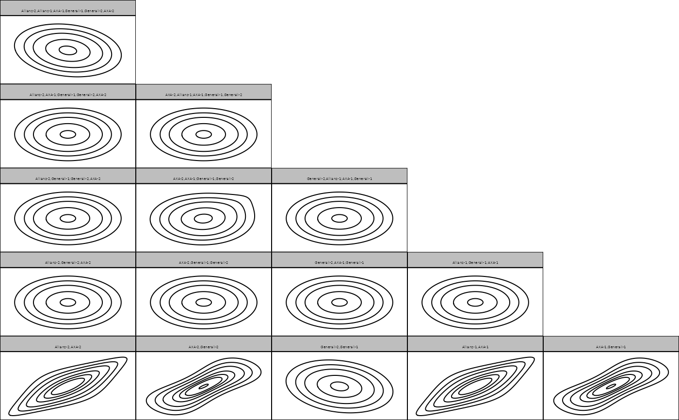
plot(fit$copula)

contour(fit$copula)

logLik(fit)
#> [1] 942.4027
#> attr(,"df")
#> [1] 12
#> attr(,"nobs")
#> [1] 100

pairs(svine_sim(500, rep = 1, fit))