Example usage of the vinereg package

This file contains the source code of an exemplary application of the D-vine copula based quantile regression approach implemented in the R-package vinereg and presented in Kraus and Czado (2017): D-vine copula based quantile regression, Computational Statistics and Data Analysis, 110, 1-18. Please, feel free to address questions to daniel.kraus@tum.de.

Load required packages

library(vinereg) 
require(ggplot2)
require(dplyr)
require(tidyr)
require(AppliedPredictiveModeling)

Data analysis

set.seed(5)

We consider the data set abalone from the UCI Machine Learning Repository (https://archive.ics.uci.edu/ml/datasets/abalone) and focus on the female sub-population. In a first application we only consider continuous variables and fit models to predict the quantiles of weight (whole) given the predictors length, diameter, and height.

Load and clean data

data(abalone, package = "AppliedPredictiveModeling")
colnames(abalone) <- c(
  "sex", "length", "diameter", "height", "whole", 
  "shucked", "viscera", "shell", "rings"
)
abalone_f <- abalone %>%
    dplyr::filter(sex == "F") %>%        # select female abalones
    dplyr::select(-sex) %>%         # remove id and sex variables
    dplyr::filter(height < max(height))  # remove height outlier

pairs(abalone_f, pch = ".")

D-vine regression models

Parametric D-vine quantile regression

We consider the female subset and fit a parametric regression D-vine for the response weight given the covariates len, diameter and height (ignoring the discreteness of some of the variables). The D-vine based model is selected sequentially by maximizing the conditional log-likelihood of the response given the covariates. Covariates are only added if they increase the (possibly AIC- or BIC-corrected) conditional log-likelihood.

We use the function vinereg() to fit a regression D-vine for predicting the response weight given the covariates length, diameter, and height. The argument family_set determines how the pair-copulas are estimated. We will only use one-parameter families and the t copula here. The selcrit argument specifies the penalty type for the conditional log-likelihood criterion for variable selection.

fit_vine_par <- vinereg(
  whole ~ length + diameter + height, 
  data = abalone_f,  
  family_set = c("onepar", "t"),
  selcrit = "aic"
)

The result has a field order that shows the selected covariates and their ranking order in the D-vine.

fit_vine_par$order

## [1] "length"   "height"   "diameter"

The field vine contains the fitted D-vine, where the first variable corresponds to the response. The object is of class "vinecop_dist" so we can use rvineocpulib’s functionality to summarize the model

summary(fit_vine_par$vine)

## # A data.frame: 6 x 11 
##  tree edge conditioned conditioning var_types family rotation  parameters df
##     1    1        1, 2                    c,c gumbel      180         5.2  1
##     1    2        2, 4                    c,c gumbel      180         2.4  1
##     1    3        4, 3                    c,c gumbel      180         2.4  1
##     2    1        1, 4            2       c,c      t        0 0.45, 21.87  2
##     2    2        2, 3            4       c,c      t        0  0.91, 4.68  2
##     3    1        1, 3         4, 2       c,c      t        0  0.31, 7.40  2
##   tau loglik
##  0.81   1629
##  0.58    672
##  0.59    709
##  0.30    147
##  0.73   1193
##  0.20     72
## 
## ---
## 1 <-> whole,   2 <-> length,   3 <-> diameter,   4 <-> height

We can also plot the contours of the fitted pair-copulas.

contour(fit_vine_par$vine)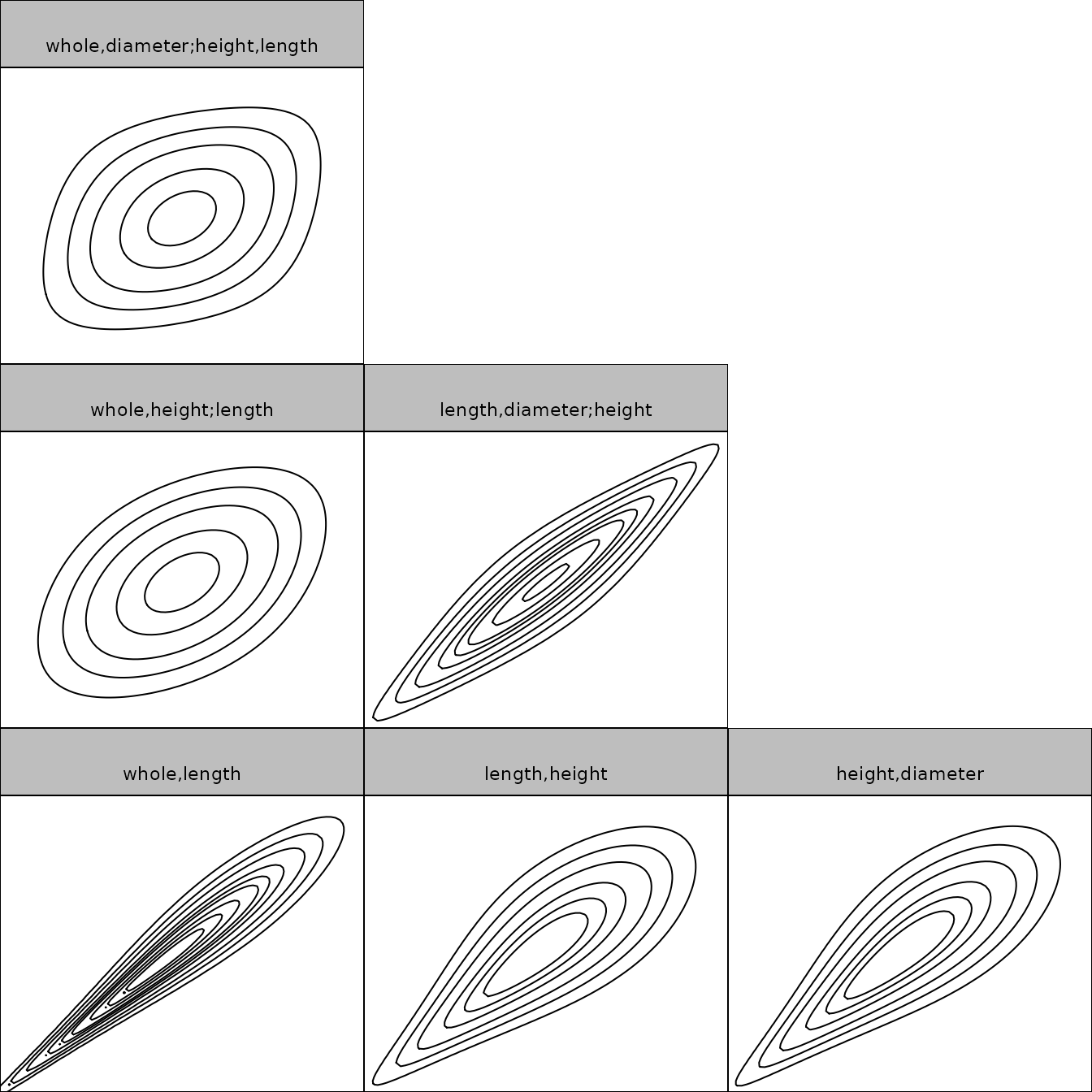

Estimation of corresponding conditional quantiles

In order to visualize the predicted influence of the covariates, we plot the estimated quantiles arising from the D-vine model at levels 0.1, 0.5 and 0.9 against each of the covariates.

# quantile levels
alpha_vec <- c(0.1, 0.5, 0.9)

We call the fitted() function on fit_vine_par to extract the fitted values for multiple quantile levels. This is equivalent to predicting the quantile at the training data. The latter function is more useful for out-of-sample predictions.

pred_vine_par <- fitted(fit_vine_par, alpha = alpha_vec)
# equivalent to:
# predict(fit_vine_par, newdata = abalone.f, alpha = alpha_vec)
head(pred_vine_par)

##         0.1       0.5       0.9
## 1 0.6717860 0.7667223 0.8716322
## 2 0.6968823 0.7903849 0.9014625
## 3 0.6794480 0.7843661 0.8914415
## 4 0.7754027 0.8800505 0.9976871
## 5 0.5950431 0.6996904 0.8273506
## 6 0.6755811 0.7729168 0.8860187

To examine the effect of the individual variables, we will plot the predicted quantiles against each of the variables. To visualize the relationship more clearly, we add a smoothed line for each quantile level. This gives an estimate of the expected effect of a variable (taking expectation with respect to all other variables).

plot_effects(fit_vine_par)

## `geom_smooth()` using method = 'gam' and formula = 'y ~ s(x, bs = "cs")'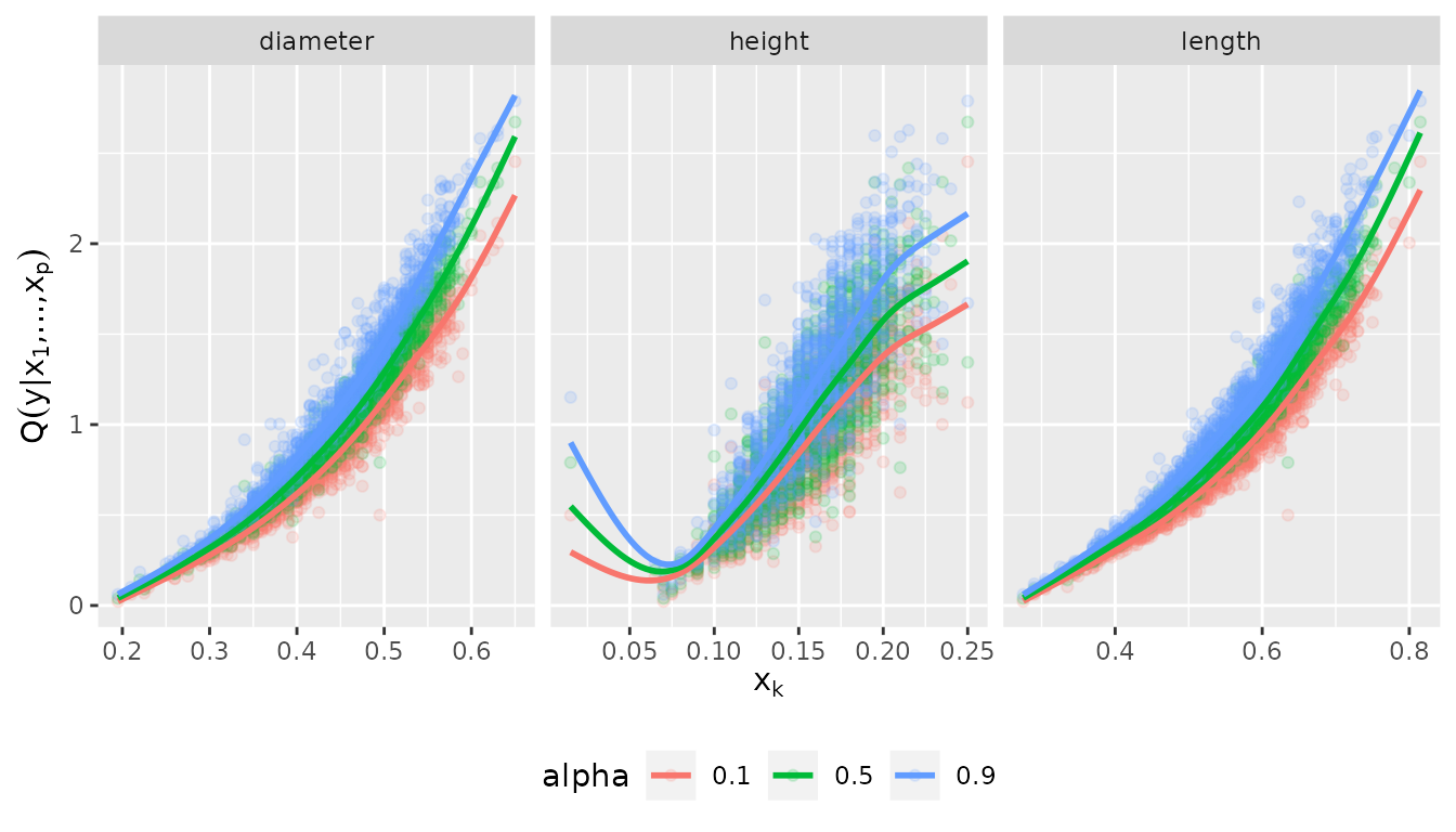

The fitted quantile curves suggest a non-linear effect of all three variables.

Comparison to the benchmark model: linear quantile regression

This can be compared to linear quantile regression:

pred_lqr <- pred_vine_par
for (a in seq_along(alpha_vec)) {
    my.rq <- quantreg::rq(
        whole ~ length + diameter + height, 
        tau = alpha_vec[a], 
        data = abalone_f
    )
    pred_lqr[, a] <- quantreg::predict.rq(my.rq)
}

plot_marginal_effects <- function(covs, preds) {
    cbind(covs, preds) %>%
        tidyr::gather(alpha, prediction, -seq_len(NCOL(covs))) %>%
        dplyr::mutate(prediction = as.numeric(prediction)) %>%
        tidyr::gather(variable, value, -(alpha:prediction)) %>%
        ggplot(aes(value, prediction, color = alpha)) +
        geom_point(alpha = 0.15) + 
        geom_smooth(method = "gam", formula = y ~ s(x, bs = "cs"), se = FALSE) + 
        facet_wrap(~ variable, scale = "free_x") +
        ylab(quote(q(y* "|" * x[1] * ",...," * x[p]))) +
        xlab(quote(x[k])) +
        theme(legend.position = "bottom")
}
plot_marginal_effects(abalone_f[, 1:3], pred_lqr)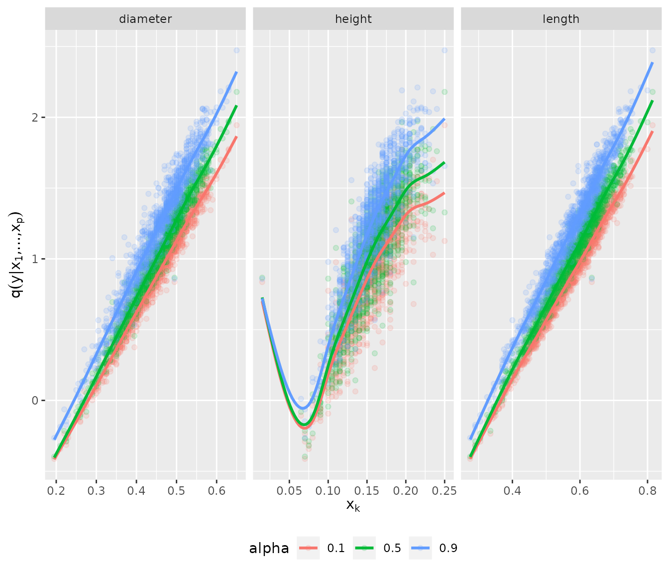

Nonparametric D-vine quantile regression

We also want to check whether these results change, when we estimate the pair-copulas nonparametrically.

fit_vine_np <- vinereg(
  whole ~ length + diameter + height,
  data = abalone_f,
  family_set = "nonpar",
  selcrit = "aic"
)
fit_vine_np

## D-vine regression model: whole | length, height, diameter 
## nobs = 1306, edf = 96.28, cll = 1208.42, caic = -2224.28, cbic = -1726.05

contour(fit_vine_np$vine)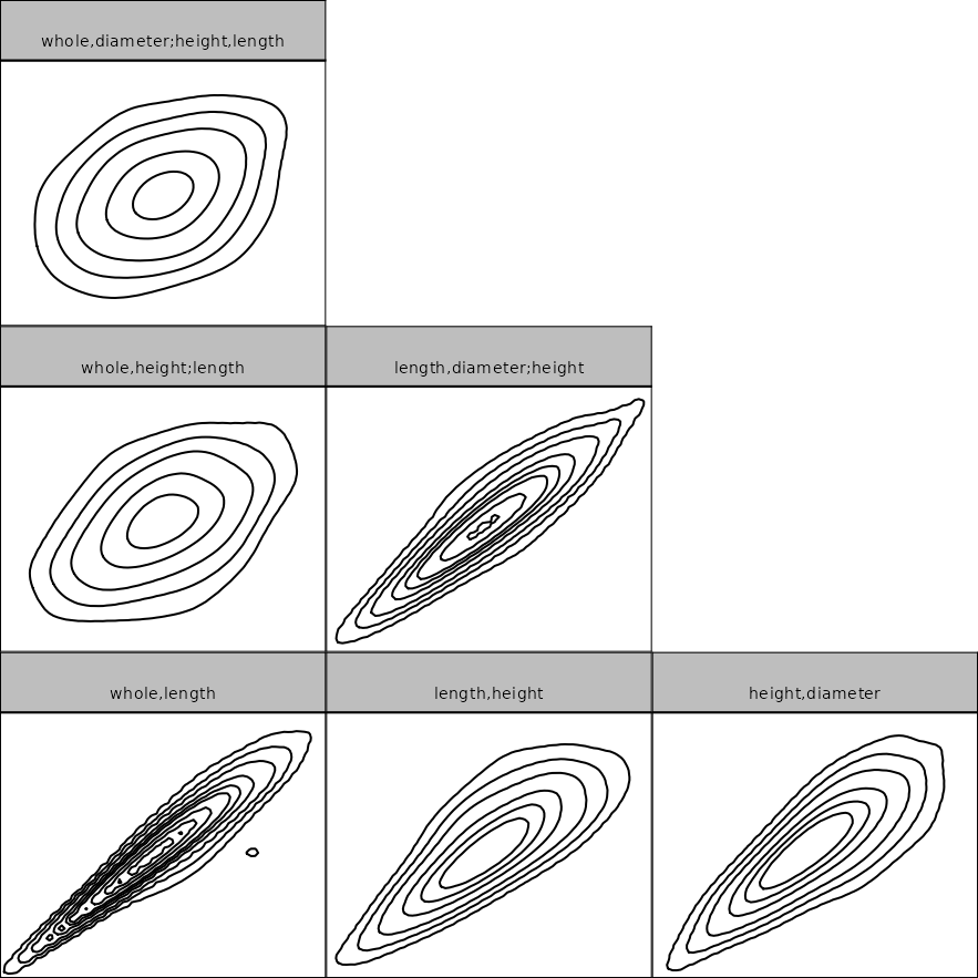

Now only the length and height variables are selected as predictors. Let’s have a look at the marginal effects.

plot_effects(fit_vine_np, var = c("diameter", "height", "length"))

## `geom_smooth()` using method = 'gam' and formula = 'y ~ s(x, bs = "cs")'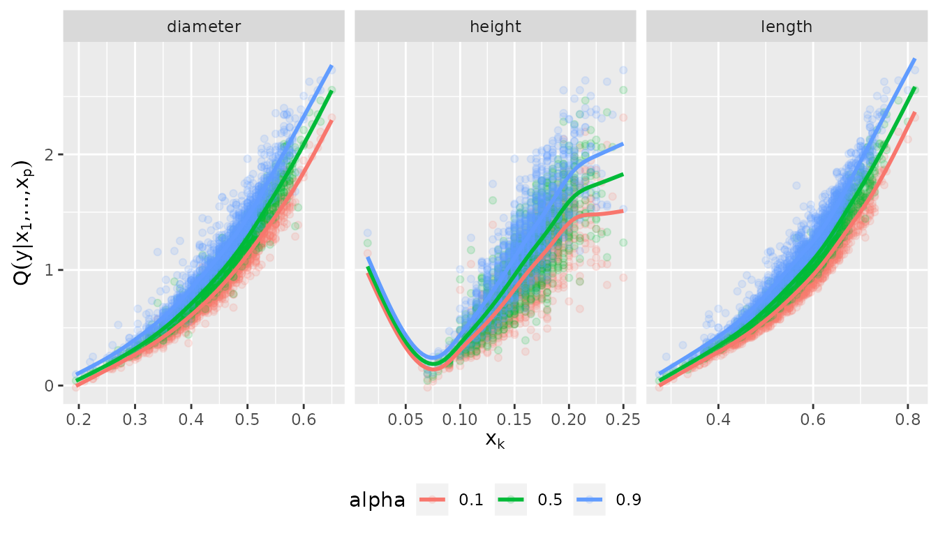

The effects look similar to the parametric one, but slightly more wiggly. Note that even the diameter was not selected as a covariate, it’s marginal effect is captured by the model. It just does not provide additional information when height and length are already accounted for.

Discrete D-vine quantile regression

To deal with discrete variables, we use the methodology of Schallhorn et al. (2017). For estimating nonparametric pair-copulas with discrete variable(s), jittering is used (Nagler, 2017).

We let vinereg() know that a variable is discrete by declaring it ordered.

abalone_f$rings <- as.ordered(abalone_f$rings)
fit_disc <- vinereg(rings ~ ., data = abalone_f, selcrit = "aic")
fit_disc

## D-vine regression model: rings | shell, shucked, whole, viscera, diameter, length, height 
## nobs = 1306, edf = 13, cll = -2737, caic = 5500.01, cbic = 5567.28

plot_effects(fit_disc)

## `geom_smooth()` using method = 'loess' and formula = 'y ~ x'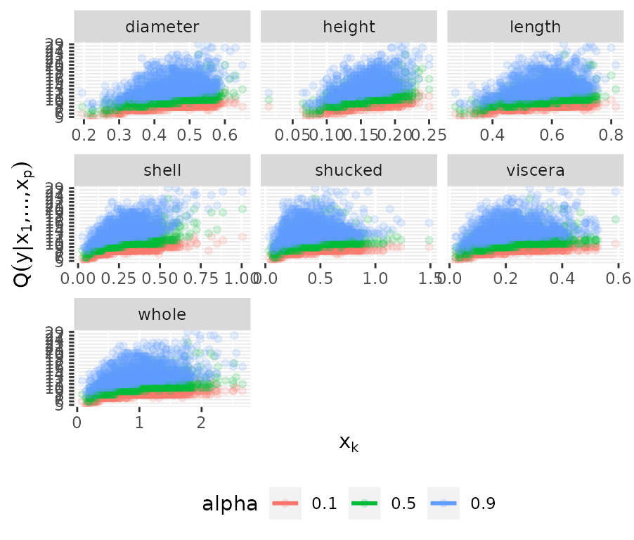

References

Kraus and Czado (2017), D-vine copula based quantile regression, Computational Statistics and Data Analysis, 110, 1-18

Nagler (2017), A generic approach to nonparametric function estimation with mixed data, Statistics & Probability Letters, 137:326–330

Schallhorn, Kraus, Nagler and Czado (2017), D-vine quantile regression with discrete variables, arXiv preprint

Daniel Kraus and Claudia Czado

September 2017