D-vine quantile regression with discrete variables: analysis of bike rental data
Dani Kraus and Thomas Nagler
November 8, 2017
Source:vignettes/bike-rental.Rmd
bike-rental.RmdPlot function for marginal effects
plot_marginal_effects <- function(covs, preds) {
    cbind(covs, preds) %>%
        tidyr::gather(alpha, prediction, -seq_len(NCOL(covs))) %>%
        dplyr::mutate(prediction = as.numeric(prediction)) %>%
        tidyr::gather(variable, value, -(alpha:prediction)) %>%
        dplyr::mutate(value = as.numeric(value)) %>%
        ggplot(aes(value, prediction, color = alpha)) +
        geom_point(alpha = 0.15) +
        geom_smooth(span = 0.5, se = FALSE) +
        facet_wrap(~ variable, scale = "free_x") +
        theme(legend.position = "none") +
        theme(plot.margin = unit(c(0, 0, 0, 0), "mm")) +
        xlab("")
}
Data preparation
Load data
##   instant     dteday season yr mnth holiday weekday workingday weathersit
## 1       1 2011-01-01      1  0    1       0       6          0          2
## 2       2 2011-01-02      1  0    1       0       0          0          2
## 3       3 2011-01-03      1  0    1       0       1          1          1
## 4       4 2011-01-04      1  0    1       0       2          1          1
## 5       5 2011-01-05      1  0    1       0       3          1          1
## 6       6 2011-01-06      1  0    1       0       4          1          1
##       temp    atemp      hum windspeed casual registered  cnt
## 1 0.344167 0.363625 0.805833 0.1604460    331        654  985
## 2 0.363478 0.353739 0.696087 0.2485390    131        670  801
## 3 0.196364 0.189405 0.437273 0.2483090    120       1229 1349
## 4 0.200000 0.212122 0.590435 0.1602960    108       1454 1562
## 5 0.226957 0.229270 0.436957 0.1869000     82       1518 1600
## 6 0.204348 0.233209 0.518261 0.0895652 88 1518 1606Show trend
ggplot(bikedata, aes(dteday, count)) +
    geom_line() +
    scale_x_date(labels = scales::date_format("%b %y")) +
    xlab("date") +
    ylab("rental count") +
    stat_smooth(method = "lm", se = FALSE, linetype = "dashed") +
    theme(plot.title = element_text(lineheight = 0.8, size = 20)) +
    theme(text = element_text(size = 18))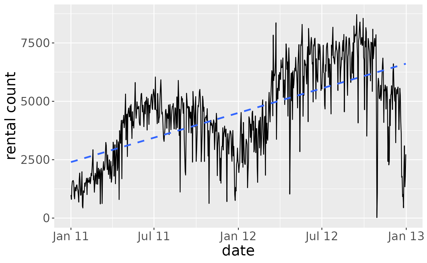
Remove trend
lm_trend <- lm(count ~ instant, data = bikedata)
trend <- predict(lm_trend)
bikedata <- mutate(bikedata, count = count / trend)
ggplot(bikedata, aes(dteday, count)) +
    geom_line() +
    scale_x_date(labels = scales::date_format("%b %y")) +
    xlab("date") +
    ylab("detrended rental count") +
    theme(plot.title = element_text(lineheight = 0.8, size = 20)) +
    theme(text = element_text(size = 18))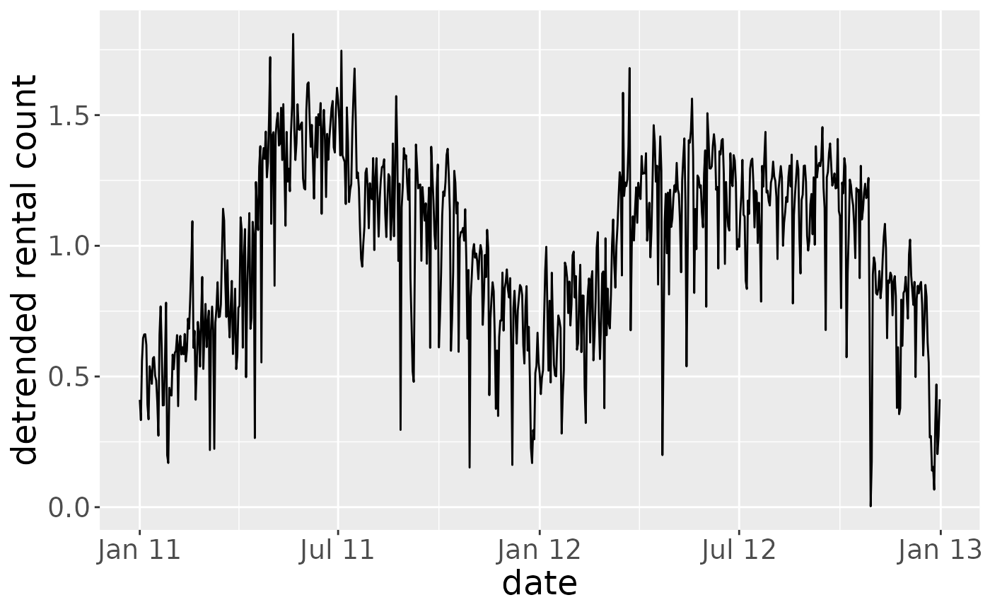
D-vine regression model
Fit model
## D-vine regression model: count | temperature, humidity, windspeed, month, weekday, weathersituation, season, workingday
## nobs = 731, edf = 83.24, cll = 448.75, caic = -731.03, cbic = -348.61
summary(fit)## var edf cll caic cbic p_value
## 1 count 9.59683 -198.076002 415.34567 459.437472 NA
## 2 temperature 21.96288 415.814280 -787.70280 -686.796245 1.057432e-161
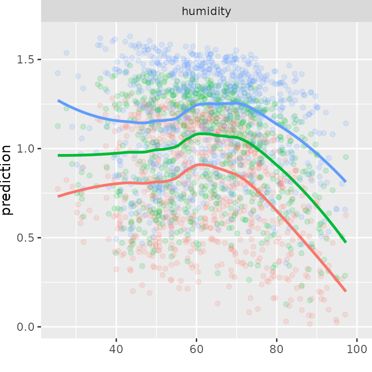
## 3 humidity 17.92242 118.868049 -201.89126 -119.548244 2.273140e-40
## 4 windspeed 1.00000 22.821902 -43.64380 -39.049391 1.418340e-11
## 5 month 16.20538 29.009883 -25.60900 48.845234 1.296498e-06
## 6 weekday 13.55004 25.682883 -24.26568 37.988828 2.604590e-06
## 7 weathersituation 1.00000 14.124718 -26.24944 -21.655023 1.066457e-07
## 8 season 1.00000 14.199792 -26.39958 -21.805170 9.868655e-08
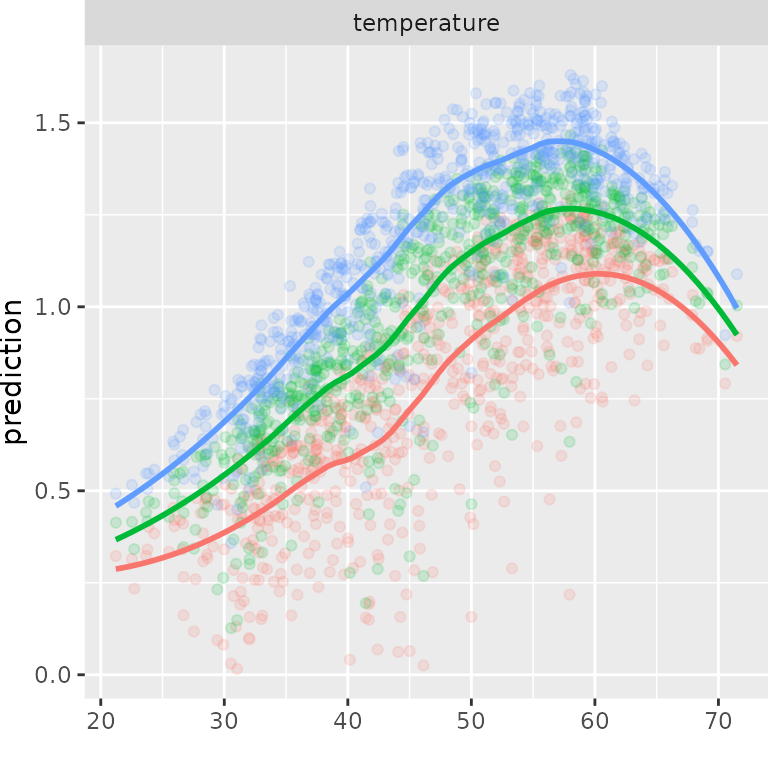
## 9 workingday 1.00000 6.309013 -10.61803 -6.023613 3.820444e-04Marginal effects
plot_marginal_effects(
    covs = select(bikedata, temperature),
    preds = pred
)
plot_marginal_effects(covs = select(bikedata, windspeed), preds = pred) 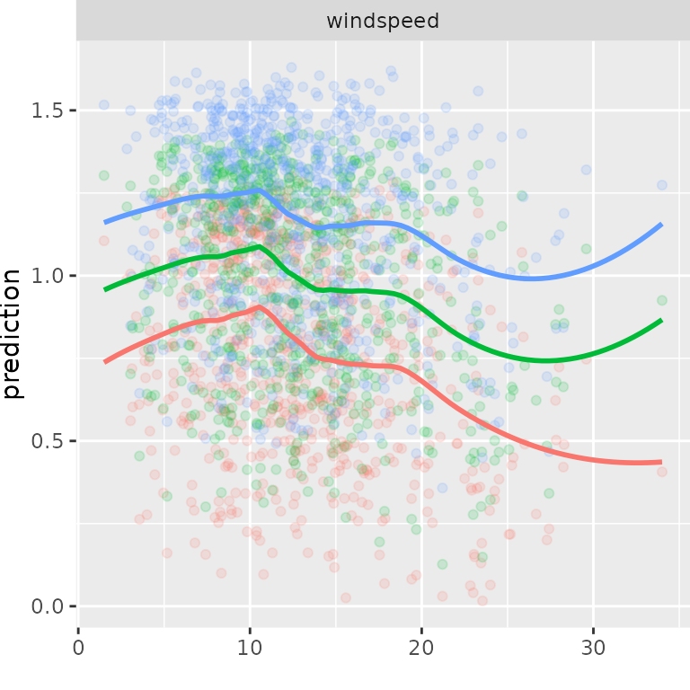
month_labs <- c("Jan","", "Mar", "", "May", "", "Jul", "", "Sep", "", "Nov", "")
plot_marginal_effects(covs = select(bikedata, month), preds = pred) +
        scale_x_discrete(limits = 1:12, labels = month_labs)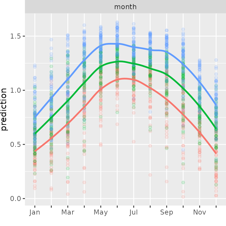
plot_marginal_effects(covs = select(bikedata, weathersituation),
                      preds = pred) +
    scale_x_discrete(limits = 1:3,labels = c("good", "medium", "bad"))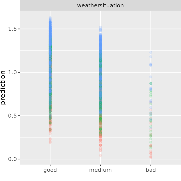
weekday_labs <- c("Mon", "Tue", "Wed", "Thu", "Fri", "Sat", "Sun")
plot_marginal_effects(covs = select(bikedata, weekday), preds = pred) +
    scale_x_discrete(limits = 1:7, labels = weekday_labs)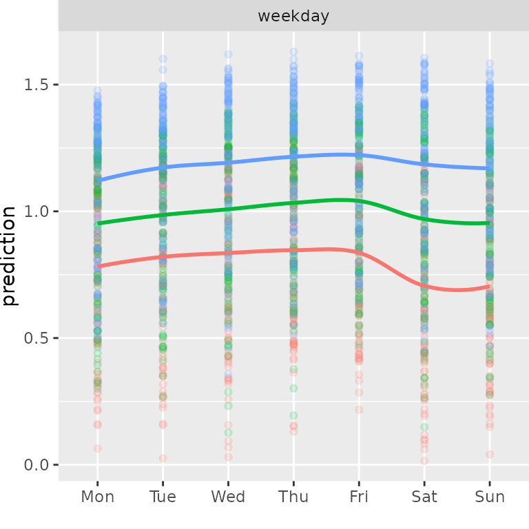
plot_marginal_effects(covs = select(bikedata, workingday), preds = pred) +
    scale_x_discrete(limits = 0:1, labels = c("no", "yes")) +
    geom_smooth(method = "lm", se = FALSE) +
    xlim(c(0, 1))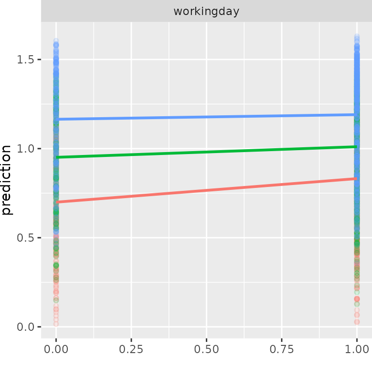
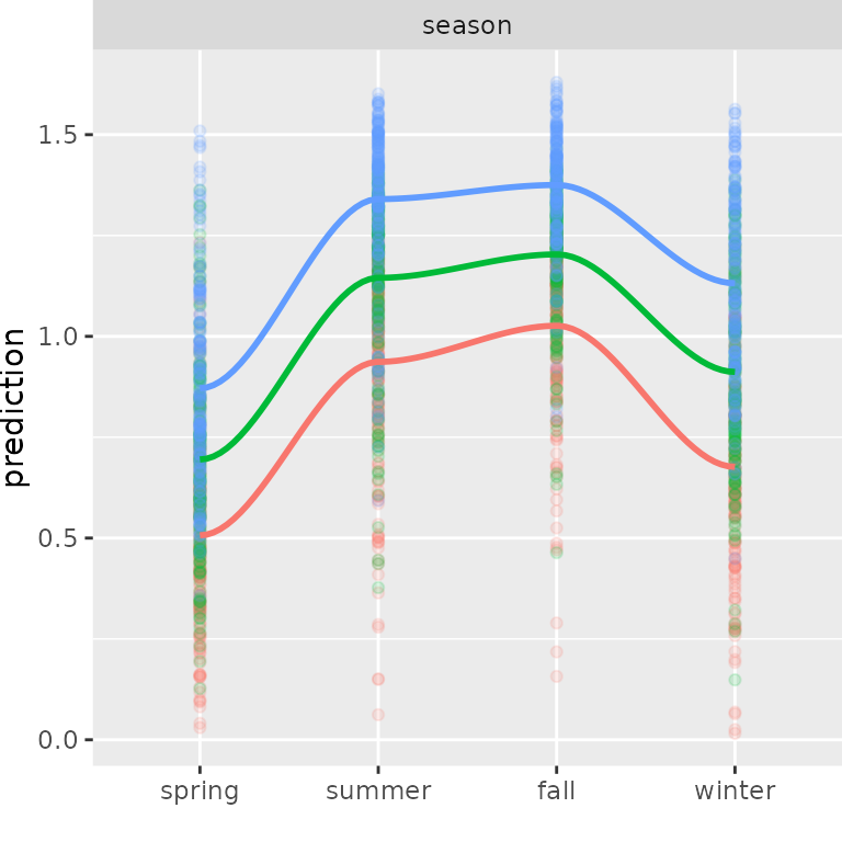
season_labs <- c("spring", "summer", "fall", "winter")
plot_marginal_effects(covs = select(bikedata, season), preds = pred) +
    scale_x_discrete(limits = 1:4, labels = season_labs)