Sequential estimation of a regression D-vine for the purpose of quantile prediction as described in Kraus and Czado (2017).
Arguments
- formula
an object of class "formula"; same as
lm().- data
data frame (or object coercible by
as.data.frame()) containing the variables in the model.- family_set
see
family_setargument ofrvinecopulib::bicop().- selcrit
selection criterion based on conditional log-likelihood.
"loglik"(default) imposes no correction; other choices are"aic"and"bic".- order
the order of covariates in the D-vine, provided as vector of variable names (after calling
vinereg:::expand_factors(model.frame(formula, data))); selected automatically iforder = NA(default).- par_1d
list of options passed to
kde1d::kde1d(), must be one value for each margin, e.g.list(xmin = c(0, 0, NaN))if the response and first covariate have non-negative support.- weights
optional vector of weights for each observation.
- cores
integer; the number of cores to use for computations.
- ...
further arguments passed to
rvinecopulib::bicop().- uscale
if TRUE, vinereg assumes that marginal distributions have been taken care of in a preliminary step.
Value
An object of class vinereg. It is a list containing the elements
- formula
the formula used for the fit.
- selcrit
criterion used for variable selection.
- model_frame
the data used to fit the regression model.
- margins
list of marginal models fitted by
kde1d::kde1d().- vine
an
rvinecopulib::vinecop_dist()object containing the fitted D-vine.- stats
fit statistics such as conditional log-likelihood/AIC/BIC and p-values for each variable's contribution.
- order
order of the covariates chosen by the variable selection algorithm.
- selected_vars
indices of selected variables.
Use
predict.vinereg() to predict conditional quantiles. summary.vinereg()
shows the contribution of each selected variable with the associated
p-value derived from a likelihood ratio test.
Details
If discrete variables are declared as ordered() or factor(), they are
handled as described in Panagiotelis et al. (2012). This is different from
previous version where the data was jittered before fitting.
References
Kraus and Czado (2017), D-vine copula based quantile regression, Computational Statistics and Data Analysis, 110, 1-18
Panagiotelis, A., Czado, C., & Joe, H. (2012). Pair copula constructions for multivariate discrete data. Journal of the American Statistical Association, 107(499), 1063-1072.
Examples
# simulate data
x <- matrix(rnorm(200), 100, 2)
y <- x %*% c(1, -2)
dat <- data.frame(y = y, x = x, z = as.factor(rbinom(100, 2, 0.5)))
# fit vine regression model
(fit <- vinereg(y ~ ., dat))
#> D-vine regression model: y | x.2, x.1, z.2, z.1
#> nobs = 100, edf = 6, cll = 62.29, caic = -112.58, cbic = -96.95
# inspect model
summary(fit)
#> var edf cll caic cbic p_value
#> 1 y 0 -217.724919 435.4498379 435.4498379 NA
#> 2 x.2 1 65.533489 -129.0669787 -126.4618085 2.393911e-30
#> 3 x.1 3 211.069184 -416.1383674 -408.3228569 3.544140e-91
#> 4 z.2 1 1.394265 -0.7885304 1.8166398 9.494126e-02
#> 5 z.1 1 2.020211 -2.0404210 0.5647492 4.442274e-02
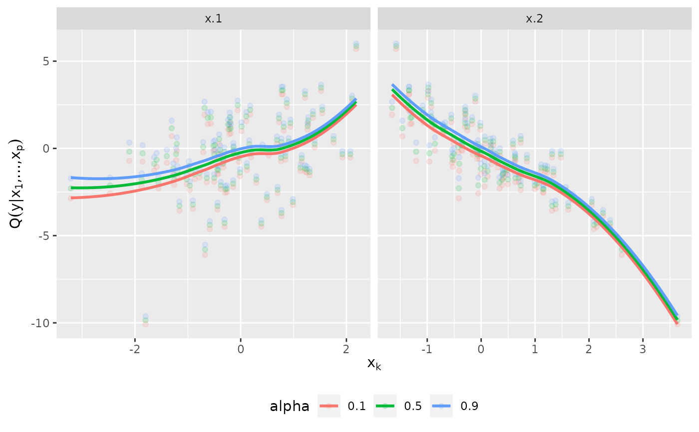
plot_effects(fit)
#> `geom_smooth()` using method = 'loess' and formula = 'y ~ x'
#> Warning: pseudoinverse used at 0.995
#> Warning: neighborhood radius 1.005
#> Warning: reciprocal condition number 0
#> Warning: There are other near singularities as well. 1.01
#> Warning: pseudoinverse used at 0.995
#> Warning: neighborhood radius 1.005
#> Warning: reciprocal condition number 0
#> Warning: There are other near singularities as well. 1.01
#> Warning: pseudoinverse used at 0.995
#> Warning: neighborhood radius 1.005
#> Warning: reciprocal condition number 0
#> Warning: There are other near singularities as well. 1.01
#> Warning: pseudoinverse used at 0.995
#> Warning: neighborhood radius 1.005
#> Warning: reciprocal condition number 0
#> Warning: There are other near singularities as well. 1.01
#> Warning: pseudoinverse used at 0.995
#> Warning: neighborhood radius 1.005
#> Warning: reciprocal condition number 0
#> Warning: There are other near singularities as well. 1.01
#> Warning: pseudoinverse used at 0.995
#> Warning: neighborhood radius 1.005
#> Warning: reciprocal condition number 0
#> Warning: There are other near singularities as well. 1.01
 # model predictions
mu_hat <- predict(fit, newdata = dat, alpha = NA) # mean
med_hat <- predict(fit, newdata = dat, alpha = 0.5) # median
# observed vs predicted
plot(cbind(y, mu_hat))
# model predictions
mu_hat <- predict(fit, newdata = dat, alpha = NA) # mean
med_hat <- predict(fit, newdata = dat, alpha = 0.5) # median
# observed vs predicted
plot(cbind(y, mu_hat))
 ## fixed variable order (no selection)
(fit <- vinereg(y ~ ., dat, order = c("x.2", "x.1", "z.1")))
#> D-vine regression model: y | x.2, x.1, z.1
#> nobs = 100, edf = 4, cll = 58.88, caic = -109.76, cbic = -99.33
## fixed variable order (no selection)
(fit <- vinereg(y ~ ., dat, order = c("x.2", "x.1", "z.1")))
#> D-vine regression model: y | x.2, x.1, z.1
#> nobs = 100, edf = 4, cll = 58.88, caic = -109.76, cbic = -99.33